5.9. Análisis de sobrevida

En esta libreta aprenderás cómo ejecutar los análisis de sobrevida más frecuentemente utilizados.

Importante

Para esta lección utilizaremos una librería nueva llamada lifelines. Puedes instalarla así:

Con UV

uv add lifelines

Con PIP

pip install lifelines

En Colab

!pip install -q lifelines

Para cualquier análisis de sobrevida necesitamos un juego de datos con al menos una columna cuantitativa de Tiempo al Evento y otra columna dicotómica de Evento Observado.

5.9.1. Librerías y datos

import scipy.stats as stats
import matplotlib.pyplot as plt
import seaborn as sns
import lifelines as ll
from lifelines.datasets import load_waltons

df = load_waltons()
df.head()

	T	E	group
0	6.0	1	miR-137
1	13.0	1	miR-137
2	13.0	1	miR-137
3	13.0	1	miR-137
4	19.0	1	miR-137

5.9.1.1. Información sobre el dataset

help(load_waltons)

Help on function load_waltons in module lifelines.datasets:

load_waltons(**kwargs)
    Genotypes and number of days survived in Drosophila. Since we work with flies, we don't need to worry about left-censoring. We know the birth date of all flies. We do have issues with accidentally killing some or if some escape. These would be right-censored as we do not actually observe their death due to "natural" causes.::

        Size: (163,3)
        Example:
             T  E    group
             6  1  miR-137
            13  1  miR-137
            13  1  miR-137
            13  1  miR-137
            19  1  miR-137

5.9.2. Exploración Visual de los datos

sns.catplot(
    data=df,
    x='group',
    y='T'
)

<seaborn.axisgrid.FacetGrid at 0x20a33122510>

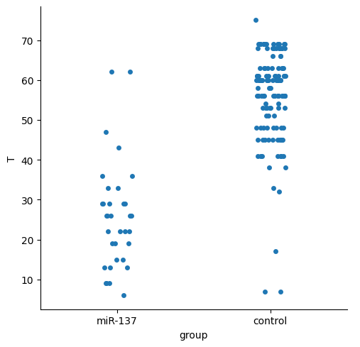
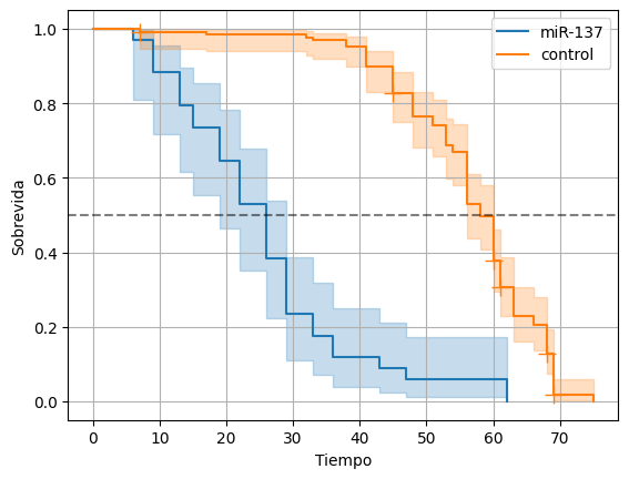
Parece que el grupo miR-137 tuvo una menor sobrevida, lo analizaremos a detalle más adelante.

Lifelines provee gráficos específicos para la exploración de los análisis de supervivencia dentro de lifelines.plotting. Utilizaremos primero ll.plotting.plot_lifetimes.

ll.plotting.plot_lifetimes(df['T'], df['E'])

c:\Users\User\Documents\coding\curso_python\.venv\Lib\site-packages\lifelines\plotting.py:773: UserWarning: For less visual clutter, you may want to subsample to less than 25 individuals.
  warnings.warn(

<Axes: >

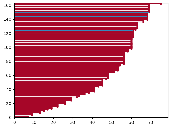
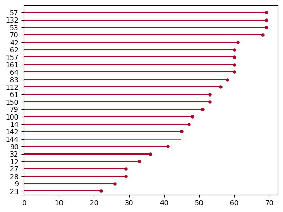
La función arroja una advertencia sobre el número de individuos, pero el gráfico es interpretable. Las líneas rojas son los eventos observados y los azules son los no observados. Veamos una muestra aleatoria de 25 individuos de este datasets.

sample = df.sample(n=25)
ll.plotting.plot_lifetimes(sample['T'], sample['E'])

<Axes: >

Podemos comenzar a analizar la sobrevida utilizando scipy, para ello, necesitamos convertir los datos a un objeto CensoredData donde especificaremos los datos observados y aquellos con algún tipo de censura.

5.9.3. Curvas de sobrevida

cd = stats.CensoredData(
    uncensored=df[df['E']==1]['T'], # seleccionamos solo a los que observamos E
    right=df[df['E']==0]['T'], # quienes desconocemos su desenlace
)
stats.ecdf(cd).sf.plot()
plt.title('Sobrevida estimada')
plt.ylabel('Tiempo')
plt.xlabel('Función de sobrevida')

Text(0.5, 0, 'Función de sobrevida')

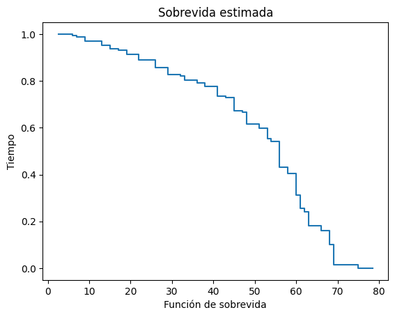
Este gráfico es simple y útil pero con limitaciones para análisis más complejos, utilizaremos lifelines.

# Primero inicializamos el estimador de Kaplan-Meier.
km = ll.KaplanMeierFitter(label='Sobrevida Waltons')
km.fit(
    durations=df['T'],
    event_observed=df['E']
)
km.plot_survival_function(
    show_censors=True
)

plt.title('Sobrevida Global')
plt.ylabel('Sobrevida')
plt.xlabel('Tiempo')
plt.axvline(km.median_survival_time_, ls='--', color='k', alpha=0.5, label='mediana')
plt.legend()
plt.grid()

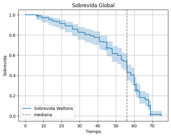
Podemos obtener información cuantitativa también.

Ahora separaremos por grupos de forma dinámica, aquí solo hay dos grupos, pero este código funcionaría incluso con más.

for group in df['group'].unique():
    km = ll.KaplanMeierFitter(label=group)
    cond = df['group'] == group
    km.fit(df[cond]['T'], df[cond]['E'])
    km.plot_survival_function(show_censors=True)
plt.grid()
plt.axhline(0.5, ls='--', color='k', alpha=0.5, label='mediana')
plt.ylabel('Sobrevida')
plt.xlabel('Tiempo')

Text(0.5, 0, 'Tiempo')

Comprobemos la significancia con la prueba de log-rank. Primero revisemos la documentación.

help(ll.statistics.logrank_test)

Help on function logrank_test in module lifelines.statistics:

logrank_test(
    durations_A,
    durations_B,
    event_observed_A=None,
    event_observed_B=None,
    t_0=-1,
    weights_A=None,
    weights_B=None,
    weightings=None,
    **kwargs
) -> lifelines.statistics.StatisticalResult
    Measures and reports on whether two intensity processes are different. That is, given two
    event series, determines whether the data generating processes are statistically different.
    The test-statistic is chi-squared under the null hypothesis. Let :math:`h_i(t)` be the hazard ratio of
    group :math:`i` at time :math:`t`, then:

    .. math::
        \begin{align}
         & H_0: h_1(t) = h_2(t) \\
         & H_A: h_1(t) = c h_2(t), \;\; c \ne 1
        \end{align}

    This implicitly uses the log-rank weights.

    Note
    -----
    - *lifelines* logrank implementation only handles right-censored data.

    - The logrank test has maximum power when the assumption of proportional hazards is true. As a consequence, if the survival curves cross, the logrank test will give an inaccurate assessment of differences.

    - This implementation is a special case of the function ``multivariate_logrank_test``, which is used internally. See Survival and Event Analysis, page 108.

    - There are only disadvantages to using the log-rank test versus using the Cox regression. See more `here <https://discourse.datamethods.org/t/when-is-log-rank-preferred-over-univariable-cox-regression/2344>`_ for a discussion. To convert to using the Cox regression:

    .. code:: python

        from lifelines import CoxPHFitter

        dfA = pd.DataFrame({'E': event_observed_A, 'T': durations_A, 'groupA': 1})
        dfB = pd.DataFrame({'E': event_observed_B, 'T': durations_B, 'groupA': 0})
        df = pd.concat([dfA, dfB])

        cph = CoxPHFitter().fit(df, 'T', 'E')
        cph.print_summary()



    Parameters
    ----------

    durations_A: iterable
        a (n,) list-like of event durations (birth to death,...) for the first population.

    durations_B: iterable
        a (n,) list-like of event durations (birth to death,...) for the second population.

    event_observed_A: iterable, optional
        a (n,) list-like of censorship flags, (1 if observed, 0 if not), for the first population.
        Default assumes all observed.

    event_observed_B: iterable, optional
        a (n,) list-like of censorship flags, (1 if observed, 0 if not), for the second population.
        Default assumes all observed.

    weights_A: iterable, optional
        case weights

    weights_B: iterable, optional
        case weights

    t_0: float, optional (default=-1)
        The final time period under observation, and subjects who experience the event after this time are set to be censored.
        Specify -1 to use all time.

    weightings: str, optional
        apply a weighted logrank test: options are "wilcoxon" for Wilcoxon (also known as Breslow), "tarone-ware"
        for Tarone-Ware, "peto" for Peto test and "fleming-harrington" for Fleming-Harrington test.
        These are useful for testing for early or late differences in the survival curve. For the Fleming-Harrington
        test, keyword arguments p and q must also be provided with non-negative values.

        Weightings are applied at the ith ordered failure time, :math:`t_{i}`, according to:
            Wilcoxon: :math:`n_i`
            Tarone-Ware: :math:`\sqrt{n_i}`
            Peto: :math:`\bar{S}(t_i)`
            Fleming-Harrington: :math:`\hat{S}(t_i)^p \times (1 - \hat{S}(t_i))^q`

            where :math:`n_i` is the number at risk just prior to time :math:`t_{i}`, :math:`\bar{S}(t_i)` is
            Peto-Peto's modified survival estimate and :math:`\hat{S}(t_i)` is the left-continuous
            Kaplan-Meier survival estimate at time :math:`t_{i}`.

    Returns
    -------

    StatisticalResult
      a StatisticalResult object with properties ``p_value``, ``summary``, ``test_statistic``, ``print_summary``

    Examples
    --------

    .. code:: python

        T1 = [1, 4, 10, 12, 12, 3, 5.4]
        E1 = [1, 0, 1,  0,  1,  1, 1]

        T2 = [4, 5, 7, 11, 14, 20, 8, 8]
        E2 = [1, 1, 1, 1,  1,  1,  1, 1]

        from lifelines.statistics import logrank_test
        results = logrank_test(T1, T2, event_observed_A=E1, event_observed_B=E2)

        results.print_summary()
        print(results.p_value)        # 0.7676
        print(results.test_statistic) # 0.0872


    See Also
    --------
    multivariate_logrank_test
    pairwise_logrank_test
    survival_difference_at_fixed_point_in_time_test

5.9.4. Log-Rank

cond = df['group'] == 'control'
controls = df[cond]
mir = df[~cond] # operador not

ll.statistics.logrank_test(
    durations_A=controls['T'],
    durations_B=mir['T'],
    event_observed_A=controls['E'],
    event_observed_B=mir['E'],
)

t_0	-1
null_distribution	chi squared
degrees_of_freedom	1
test_name	logrank_test

	test_statistic	p	-log2(p)
0	122.25	<0.005	91.99

5.9.5. Sobrevida condicional

La sobrevida condicional responde a preguntas como:

“¿Cuál es la probabilidad de que un individuo sobreviva 10 días más, dado que ya ha sobrevivido los primeros 20?”

Matemáticamente, se define como:

\[ S(t \mid t > t_0) = \frac{S(t)}{S(t_0)} \]

donde ( S(t) ) es la función de sobrevida acumulada, y ( t_0 ) es el tiempo a partir del cual se condiciona la probabilidad de seguir sobreviviendo.

Esto es útil en seguimiento clínico, por ejemplo, para pacientes que ya han superado una etapa crítica y queremos estimar su pronóstico futuro.

5.9.5.1. Ejemplo global

Supongamos que queremos saber cuál es la probabilidad de que un individuo sobreviva al menos 10 días más, dado que ya ha sobrevivido 15 días.

# Ajustamos el modelo Kaplan-Meier
km = ll.KaplanMeierFitter()
km.fit(durations=df['T'], event_observed=df['E'])

# Obtenemos la sobrevida en t = 15 y t = 25
S_15, S_25 = km.survival_function_at_times([15, 25])

# Sobrevida condicional: probabilidad de sobrevivir hasta 25, dado que llegó a 15
cond_surv = S_25 / S_15
print(f"Probabilidad de sobrevivir 10 días más (de 15 a 25), dado que llegó a 15: {cond_surv:.3f}")

Probabilidad de sobrevivir 10 días más (de 15 a 25), dado que llegó a 15: 0.947

5.9.6. Ejercicios

1. Explora las opciones disponibles en lifelines.datasets y prueba tus conocimientos con estos datasets.

2. El objeto cd de scipy ofrece un interfaz sencilla para obtener información de sobrevida. Revisa la documentación para ver qué puede hacer. Te sugiero iniciar por aquí y aquí.

3. Compara la sobrevida condicionada entre los controles y el grupo de estudio.

4. Revisa la documentación de lifelines para ver otros ejemplos.

5. Aplica lo aprendido con tus propios datos.