6.2. Pruebas T, parte 1#
Para realizar las pruebas t con inferencia Bayesiana el método más sencillo es utilizar pingouin que produce por defecto factores de Bayes (BF) además del valor p frecuentista.
6.2.1. Librerías y datos#
Utilizaremos los palmer penguins que ya hemos revisado en el curso.
import pandas as pd
import pingouin as pg
import seaborn as sns

data = pg.read_dataset('penguins')
data.head()
| species | island | bill_length_mm | bill_depth_mm | flipper_length_mm | body_mass_g | sex | |
|---|---|---|---|---|---|---|---|
| 0 | Adelie | Biscoe | 37.8 | 18.3 | 174.0 | 3400.0 | female |
| 1 | Adelie | Biscoe | 37.7 | 18.7 | 180.0 | 3600.0 | male |
| 2 | Adelie | Biscoe | 35.9 | 19.2 | 189.0 | 3800.0 | female |
| 3 | Adelie | Biscoe | 38.2 | 18.1 | 185.0 | 3950.0 | male |
| 4 | Adelie | Biscoe | 38.8 | 17.2 | 180.0 | 3800.0 | male |
6.2.2. Visualización de grupos.#
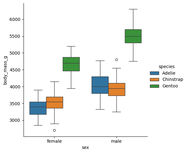
Probemos la forma más sencilla del análisis comparando body_mass_g de acuerdo a la variable sex.
clean_data = data.dropna(subset=['body_mass_g', 'sex'])

sns.catplot(clean_data, x='sex', y='body_mass_g', hue='species', kind='box')
<seaborn.axisgrid.FacetGrid at 0x1862d9925d0>
sns.displot(
    clean_data,
    x='body_mass_g',
    hue='sex',
    kind='kde',
    col='species'
)
<seaborn.axisgrid.FacetGrid at 0x18630c1a210>
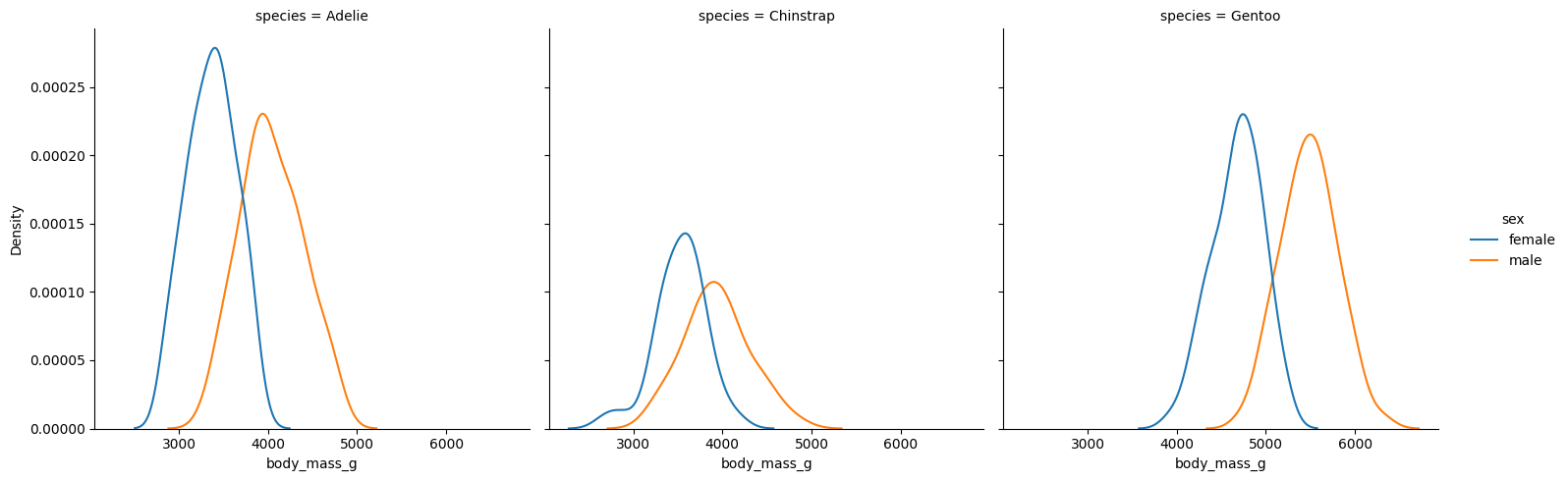
Vemos que efectivamente hay una diferencia en peso corporal con respecto al sexo y a la especie. Probemos ahora el análisis.
Antes de ejecutar el análisis, conviene leer la documentación de la función. Te sugiero leerlo en la página de pingouin, pero también podemos verlo con la función help.
help(pg.ttest)
Help on function ttest in module pingouin.parametric:

ttest(
    x,
    y,
    paired=False,
    alternative='two-sided',
    correction='auto',
    r=0.707,
    confidence=0.95
)
    T-test.

    Parameters
    ----------
    x : array_like
        First set of observations.
    y : array_like or float
        Second set of observations. If ``y`` is a single value, a one-sample
        T-test is computed against that value (= "mu" in the t.test R
        function).
    paired : boolean
        Specify whether the two observations are related (i.e. repeated
        measures) or independent.
    alternative : string
        Defines the alternative hypothesis, or tail of the test. Must be one of
        "two-sided" (default), "greater" or "less". Both "greater" and "less" return one-sided
        p-values. "greater" tests against the alternative hypothesis that the mean of ``x``
        is greater than the mean of ``y``.
    correction : string or boolean
        For unpaired two sample T-tests, specify whether or not to correct for
        unequal variances using Welch separate variances T-test. If 'auto', it
        will automatically uses Welch T-test when the sample sizes are unequal,
        as recommended by Zimmerman 2004.
    r : float
        Cauchy scale factor for computing the Bayes Factor.
        Smaller values of r (e.g. 0.5), may be appropriate when small effect
        sizes are expected a priori; larger values of r are appropriate when
        large effect sizes are expected (Rouder et al 2009).
        The default is 0.707 (= :math:`\sqrt{2} / 2`).
    confidence : float
        Confidence level for the confidence intervals (0.95 = 95%)

        .. versionadded:: 0.3.9

    Returns
    -------
    stats : :py:class:`pandas.DataFrame`

        * ``'T'``: T-value
        * ``'dof'``: degrees of freedom
        * ``'alternative'``: alternative of the test
        * ``'p-val'``: p-value
        * ``'CI95%'``: confidence intervals of the difference in means
        * ``'cohen-d'``: Cohen d effect size
        * ``'BF10'``: Bayes Factor of the alternative hypothesis
        * ``'power'``: achieved power of the test ( = 1 - type II error)

    See also
    --------
    mwu, wilcoxon, anova, rm_anova, pairwise_tests, compute_effsize

    Notes
    -----
    Missing values are automatically removed from the data. If ``x`` and
    ``y`` are paired, the entire row is removed (= listwise deletion).

    The **T-value for unpaired samples** is defined as:

    .. math::

        t = \frac{\overline{x} - \overline{y}}
        {\sqrt{\frac{s^{2}_{x}}{n_{x}} + \frac{s^{2}_{y}}{n_{y}}}}

    where :math:`\overline{x}` and :math:`\overline{y}` are the sample means,
    :math:`n_{x}` and :math:`n_{y}` are the sample sizes, and
    :math:`s^{2}_{x}` and :math:`s^{2}_{y}` are the sample variances.
    The degrees of freedom :math:`v` are :math:`n_x + n_y - 2` when the sample
    sizes are equal. When the sample sizes are unequal or when
    :code:`correction=True`, the Welch–Satterthwaite equation is used to
    approximate the adjusted degrees of freedom:

    .. math::

        v = \frac{(\frac{s^{2}_{x}}{n_{x}} + \frac{s^{2}_{y}}{n_{y}})^{2}}
        {\frac{(\frac{s^{2}_{x}}{n_{x}})^{2}}{(n_{x}-1)} +
        \frac{(\frac{s^{2}_{y}}{n_{y}})^{2}}{(n_{y}-1)}}

    The p-value is then calculated using a T distribution with :math:`v`
    degrees of freedom.

    The T-value for **paired samples** is defined by:

    .. math:: t = \frac{\overline{x}_d}{s_{\overline{x}}}

    where

    .. math:: s_{\overline{x}} = \frac{s_d}{\sqrt n}

    where :math:`\overline{x}_d` is the sample mean of the differences
    between the two paired samples, :math:`n` is the number of observations
    (sample size), :math:`s_d` is the sample standard deviation of the
    differences and :math:`s_{\overline{x}}` is the estimated standard error
    of the mean of the differences. The p-value is then calculated using a
    T-distribution with :math:`n-1` degrees of freedom.

    The scaled Jeffrey-Zellner-Siow (JZS) Bayes Factor is approximated
    using the :py:func:`pingouin.bayesfactor_ttest` function.

    Results have been tested against JASP and the `t.test` R function.

    References
    ----------
    * https://www.itl.nist.gov/div898/handbook/eda/section3/eda353.htm

    * Delacre, M., Lakens, D., & Leys, C. (2017). Why psychologists should
      by default use Welch’s t-test instead of Student’s t-test.
      International Review of Social Psychology, 30(1).

    * Zimmerman, D. W. (2004). A note on preliminary tests of equality of
      variances. British Journal of Mathematical and Statistical
      Psychology, 57(1), 173-181.

    * Rouder, J.N., Speckman, P.L., Sun, D., Morey, R.D., Iverson, G.,
      2009. Bayesian t tests for accepting and rejecting the null
      hypothesis. Psychon. Bull. Rev. 16, 225–237.
      https://doi.org/10.3758/PBR.16.2.225

    Examples
    --------
    1. One-sample T-test.

    >>> from pingouin import ttest
    >>> x = [5.5, 2.4, 6.8, 9.6, 4.2]
    >>> ttest(x, 4).round(2)
              T  dof alternative  p-val         CI95%  cohen-d   BF10  power
    T-test  1.4    4   two-sided   0.23  [2.32, 9.08]     0.62  0.766   0.19

    2. One sided paired T-test.

    >>> pre = [5.5, 2.4, 6.8, 9.6, 4.2]
    >>> post = [6.4, 3.4, 6.4, 11., 4.8]
    >>> ttest(pre, post, paired=True, alternative='less').round(2)
               T  dof alternative  p-val          CI95%  cohen-d   BF10  power
    T-test -2.31    4        less   0.04  [-inf, -0.05]     0.25  3.122   0.12

    Now testing the opposite alternative hypothesis

    >>> ttest(pre, post, paired=True, alternative='greater').round(2)
               T  dof alternative  p-val         CI95%  cohen-d  BF10  power
    T-test -2.31    4     greater   0.96  [-1.35, inf]     0.25  0.32   0.02

    3. Paired T-test with missing values.

    >>> import numpy as np
    >>> pre = [5.5, 2.4, np.nan, 9.6, 4.2]
    >>> post = [6.4, 3.4, 6.4, 11., 4.8]
    >>> ttest(pre, post, paired=True).round(3)
                T  dof alternative  p-val          CI95%  cohen-d   BF10  power
    T-test -5.902    3   two-sided   0.01  [-1.5, -0.45]    0.306  7.169  0.073

    Compare with SciPy

    >>> from scipy.stats import ttest_rel
    >>> np.round(ttest_rel(pre, post, nan_policy="omit"), 3)
    array([-5.902,  0.01 ])

    4. Independent two-sample T-test with equal sample size.

    >>> np.random.seed(123)
    >>> x = np.random.normal(loc=7, size=20)
    >>> y = np.random.normal(loc=4, size=20)
    >>> ttest(x, y)
                   T  dof alternative         p-val         CI95%   cohen-d       BF10  power
    T-test  9.106452   38   two-sided  4.306971e-11  [2.64, 4.15]  2.879713  1.366e+08    1.0

    5. Independent two-sample T-test with unequal sample size. A Welch's T-test is used.

    >>> np.random.seed(123)
    >>> y = np.random.normal(loc=6.5, size=15)
    >>> ttest(x, y)
                   T        dof alternative     p-val          CI95%   cohen-d   BF10     power
    T-test  1.996537  31.567592   two-sided  0.054561  [-0.02, 1.65]  0.673518  1.469  0.481867

    6. However, the Welch's correction can be disabled:

    >>> ttest(x, y, correction=False)
                   T  dof alternative     p-val          CI95%   cohen-d   BF10     power
    T-test  1.971859   33   two-sided  0.057056  [-0.03, 1.66]  0.673518  1.418  0.481867

    Compare with SciPy

    >>> from scipy.stats import ttest_ind
    >>> np.round(ttest_ind(x, y, equal_var=True), 6)  # T value and p-value
    array([1.971859, 0.057056])
condition = (clean_data['sex'] == 'female')
fem = clean_data[condition]['body_mass_g']
male = clean_data[~condition]['body_mass_g'] # operador not

# prueba t

pg.ttest(fem, male)
| T | dof | alternative | p-val | CI95% | cohen-d | BF10 | power | |
|---|---|---|---|---|---|---|---|---|
| T-test | -8.554537 | 323.895881 | two-sided | 4.793891e-16 | [-840.58, -526.25] | 0.936205 | 1.142e+13 | 1.0 |
El resultado incluye el estadístico t, los grados de libertad, el tipo de hipótesis, el valor p, el intervalo de confianza para la diferencia de medias, el tamaño del efecto (d de Cohen), el factor de Bayes \(BF_{10}\), y el poder post-hoc del análisis.
En este caso, se utilizó un valor por defecto de \(r=0.707\), que corresponde al parámetro de escala de una distribución Cauchy centrada en 0, utilizada como prior sobre el tamaño del efecto bajo la hipótesis alternativa.
El factor r, bajo la distribución Cauchy del tamaño del efecto se define con la siguiente fórmula, el factor por defecto fue descrito por Rouder (2009) y se utiliza en muchas implementaciones en Python, R, JASP, etc. Se calcula de la siguiente forma:
Rouder, J.N., Speckman, P.L., Sun, D., Morey, R.D., Iverson, G., Bayesian t tests for accepting and rejecting the null hypothesis. Psychon. Bull. Rev. 16, 225–237. https://doi.org/10.3758/PBR.16.2.225
Pero si contáramos con estudios previos que sugirieran un tamaño del efecto diferente, el análisis debería contemplarlo. Analicemos la diferencia global del peso entre los Chinstrap y los Adelie.
condition = (clean_data['sex'] == 'female') & (clean_data['species'] != 'Gentoo')
sns.displot(clean_data[condition], x='body_mass_g', hue='species', kind='kde')
<seaborn.axisgrid.FacetGrid at 0x1863346a990>
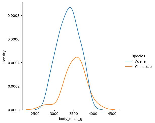
Vemos que la diferencia es minúscula. Veamos cómo cambia el factor de Bayes con diferentes valores de r
chinstrap = clean_data[clean_data['species'] == 'Chinstrap']['body_mass_g']
adelie = clean_data[clean_data['species'] == 'Adelie']['body_mass_g']


result = pd.concat([
    pg.ttest(adelie, chinstrap, r=r).assign(r=r)
    for r in [0.1, 0.5, 0.707, 1]
])

result
| T | dof | alternative | p-val | CI95% | cohen-d | BF10 | power | r | |
|---|---|---|---|---|---|---|---|---|---|
| T-test | -0.44793 | 154.032619 | two-sided | 0.654833 | [-145.66, 91.82] | 0.06168 | 0.651 | 0.070266 | 0.100 |
| T-test | -0.44793 | 154.032619 | two-sided | 0.654833 | [-145.66, 91.82] | 0.06168 | 0.238 | 0.070266 | 0.500 |
| T-test | -0.44793 | 154.032619 | two-sided | 0.654833 | [-145.66, 91.82] | 0.06168 | 0.175 | 0.070266 | 0.707 |
| T-test | -0.44793 | 154.032619 | two-sided | 0.654833 | [-145.66, 91.82] | 0.06168 | 0.126 | 0.070266 | 1.000 |
Nota
El código anterior utiliza una comprensión de lista, puedes ver cómo funciona aquí.
Observamos que el valor p no alcanza significación estadística, y que el \(BF_{10}\) proporciona evidencia moderada a fuerte a favor de la hipótesis nula \(H_0: \text{Peso}{\text{Adelie}} = \text{Peso}{\text{Chinstrap}}\), incluso al usar un valor ingenuo de \(r = 0.5\).
6.2.3. Interpretación de \(BF_{10}\)#
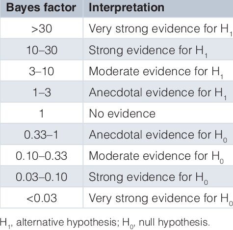
Figura 6.1 Tabla de referencia para los diferentes puntos de corte del Factor de Bayes.#
Imagen reproducida bajo los términos de la licencia CC BY 4.0.
Garnett, Claire & Michie, Susan & West, Robert & Brown, Jamie. (2019). Updating the evidence on the effectiveness of the alcohol reduction app, Drink Less: using Bayes factors to analyse trial datasets supplemented with extended recruitment. F1000Research. 8. 114. 10.12688/f1000research.17952.2.
6.2.4. Ejercicios#
Aplica lo aprendido con tus propios datos.
Analiza la diferencia en el ancho del pico de acuerdo al sexo.